Generative Learning in VLSI Design for Manufacturability: Current Status and Future Directions

Research Article Archive • Versions 1 Vol 2 (4) : 19020401 2019

Mohamed Baker Alawieh, Yibo Lin, Wei Ye, David Z. Pan

DOI: 10.33079/jomm.19020401

： 2019 - 10 - 16

： 2019 - 12 - 13

： 2019 - 12 - 25

3331 61 0

Abstract & Keywords

Abstract: With the continuous scaling of integrated circuit technologies, design for manufacturability (DFM) is becoming more critical, yet more challenging. Alongside, recent advances in machine learning have provided a new computing paradigm with promising applications in VLSI manufacturability. In particular, generative learning - regarded among the most interesting ideas in present-day machine learning - has demonstrated impressive capabilities in a wide range of applications. This paper surveys recent results of using generative learning in VLSI manufacturing modeling and optimization. Specifically, we examine the unique features of generative learning that have been leveraged to improve DFM efficiency in an unprecedented way; hence, paving the way to a new data-driven DFM approach. The state-of-the-art methods are presented, and challenges/opportunities are discussed.

Keywords: Design for Manufacturability; Generative Learning; Machine Learning; Lithography

1. Introduction

Recent advances in machine learning have dramatically altered the perception of computing through providing the ability to learn without traditional explicit programming. With its far-reaching data-driven perspective for problem solving, experts in all fields of study have been re-examining, through the new lens of machine learning, different problems that traditional computing paradigms were ill-equipped to handle. In fact, with new successes and adoption in many domains, machine learning has been rapidly infiltrating into diverse fields such as medicine^[1,2], finance^[3], and automation in all its aspects^[4–7].

With the thrust in machine learning (ML) research still gaining momentum, new models are being continuously developed in both the supervised and unsupervised areas. Traditionally, regression and classification models have been the most prominent learning models with applications in many fields being cast into either of them^[8]. Recently, new learning paradigms have emerged, and thus provided new prospects for machine learning. Among these paradigms is generative learning which has been considered one of the most interesting ideas in the last decade in machine learning^{[9, 10]}.

With generative learning, the role of machine learning models has been flipped from mere data consumers to data generators. In fact, models that started as a means for data compression and feature extraction^[11] have quickly emerged to generative models capable of producing quality samples based on a learned distribution ^{[9, 12]}. Despite its original intended target of generating fake images that can fool traditional machine learning models (from which the term adversary comes), applications of state-of-the-art generative adversarial networks (GANs) have demonstrated that such adversary can be reconciled and put towards a good use; thus, turning adversary into a powerful tool.

In its essence, generative learning targets developing a model that is capable of learning the distribution of a given data set with the intent of generating new samples from it^[9]. This can be useful in several applications where data is scarce and available datasets are insufficient for supervised learning tasks such as regression and classification^[13]. In this aspect, generative learning is viewed as a data preparation tool which is critical in machine learning. However, recently, generative models stepped beyond this limit to claim the central role as stand-alone models capable of performing complex tasks, and nowhere is this more evident than in conditional GANs (CGANs) that have been adopted in different applications. Unlike conventional GANs that target stochastic sample generation, a CGAN is perceived as a translator; i.e., given a sample in a particular domain, it targets translating it to another. A simple example is image coloring where black and white images are colored using a trained CGAN. In this sense, a CGAN is viewed as a powerful tool that can replace many time-consuming processes such as medical image synthesis^[14] and lithography simulation^[15].

In the midst of the machine learning revolution, Electronic Design Automation (EDA), as most other fields of research, has adopted the recent advances to address challenges in the field^[4]. In particular, generative learning has been widely adopted in many applications to improve the efficiency of the design process. These applications span different domains with particular success in physical design automation^[16–20] and design for manufacturability (DFM) related applications^{[15, 21–25]}. In these applications, generative learning has stepped out of the conventional frame to act as a data-driven optimizer or simulator that can significantly speedup design closure. This in fact paves the way for a new paradigm of design automation with limited dependence on expensive traditional simulation and optimization tools.

In this paper, we review recent applications of generative learning in the field of DFM. Here, we present the successful adoption of this learning scheme in DFM while shedding light on the new paradigm such scheme has introduced into the field. We first review the necessary background about generative learning in Section 2 and then present its applications in DFM in Section 3. In Section 4, we reflect on the impact of these applications and possible future works. Conclusions are presented in Section 5.

2. Generative Learning Background

In this section, we review the background of the state-of-the-art generative learning models that have been recently adopted to address challenges in DFM. In particular, we first present different types of autoencoders which are typically used for data generation; i.e., the very core target of these models. Next, we review GAN models which stepped out of their core domain in modeling and generation to claim the roles of simulators and optimizers which are critical and tedious in many DFM applications.

2.1 Autoencoders

Autoencoders (AEs) have been traditionally used as data compression tools for dimensionality reduction and feature learning^{[26, 27]}. These models are lossy compression tools that are leaned from data and are data specific. In other words, an AE can compress data similar to that seen in the training process while incurring some degradation when decompressing the input. These features of AE rank it among the most used feature extraction and dimensionality reduction tools^[12].

In principle, an AE is composed of two functions typically implemented using neural networks: an encoder function \(f\) and a decoder function \(h\). Given a dataset {\({x}_{i}\) : i = 1, . . . , N}, AE can be used to obtain a low dimensional latent space representation {\({z}_{i}\): i = 1, . . . , N} of the input samples ^{[12, 26]}. Hence, the objective is to learn the two mapping functions \(f:x\to z\) and \(h:z\to x\) . Typically, the dimension of \({z}_{i}\) is significantly smaller than that of \({x}_{i}\) Hence, the low-level embedding can be used as a feature vector when developing complex supervised machine learning models such as image classification or object detection^[27].

From a model perspective, an AE is an unsupervised model that implements the encoding function \(f\) as a down sampling stream that starts from the input \(x\) to generate the latent representation \(z\), and \(g\) as an upsampling one that takes \(z\) as an input to regenerate \(x\) as shown in Fig. 1(a) ^[12]. The objective is to generate an output \({\hat{x}}_{i}\) that is ideally equal to \(x\) and practically as close to it as possible. Mathematically, the objective of the training process is to minimize the following loss function:

\[{\mathcal{L}}_{AE}={\sum }_{i=1}^{N}l\left({x}_{i},{\hat{x}}_{i}\right),\qquad \qquad \qquad \qquad \text{(1)}\]

where \(l\)(\({x}_{i}\),\( {\hat{x}}_{i}\)) can be an l₂ -norm distance, pixel-wise cross entropy for images^[27], or any other function that can capture the discrepancy between \({x}_{i}\) and \({\hat{x}}_{i}\).

Figure 1. The architecture for (a) an autoencoder and (b) a variational autoencoder.

While an AE is adequate for data compression and feature extraction, generating synthetic data samples using it is not trivial since it does not explicitly learn the probability distribution representing the data^[12]. On the other hand, variational auto-encoders (VAEs) were developed to model this distribution; hence, presenting a generative model framework that allows sampling new synthetic data from the learned distribution ^{[11, 12, 27]}. The architecture of a VAE is very similar to that of an AE with the main difference lying in the latent space representation. Instead of training the encoder function \(f\) to generate the latent representation \(z\), it is trained to learn the distribution of \(z\) through the parameters \(μ\) and \(\sigma \) as shown in Fig. 1(b). Then, \(z\) is sampled from the learned distribution with some additive noise before being fed to the decoder network which works in the same fashion as in an AE. Mathematically, \(z\) can be obtained as follows^[11]:

\[z=\mu +{\sigma }^{1/2}\cdot ϵ, \text{where } ϵ \in \mathcal{N}\left(0,I\right) \qquad \qquad \text{ (2)} \]

Moreover, to govern the distribution learning process, the objective function is adjusted to include a KL-divergence term that captures the difference between the prior distribution of \(z\), \(P\left(z\right)\), and that learned after seeing the samples \(x\), \(Q\left(z|x\right)\)^[11] . The new loss function for the VAE model is given as:

\[{\mathcal{L}}_{VAE}={\mathcal{L}}_{AE}+\lambda \bullet {\mathcal{D}}_{KL}\left[Q\left(z|x\right)||P\left(z\right)\right] \qquad \qquad \qquad \qquad \text{(3)}\]

where \({\mathcal{D}}_{KL}\left[Q||P\right]\) represents the KL-divergence between distributions \(Q\) and \(P\) and \(\lambda \) is a hyper parameter used to tune the importance of the two different loss terms.

2.2 Generative Adversarial Networks

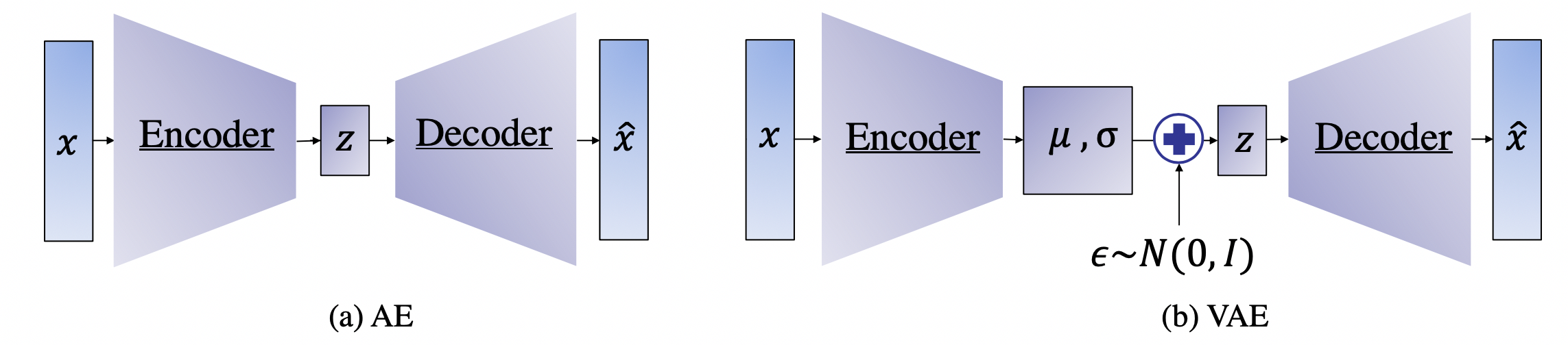
While the VAE is a generative model that is capable of producing new samples from a learned data distribution, its main objective is to learn the latent space representation and the corresponding distribution. Generative adversarial networks (GANs) are explicitly set up to optimize for the generative tasks^[9]. In their essence, GANs were proposed as generative models that learn a mapping from a random noise vector \(z\) to an output \(y\), \(G: z \to y\)^[9] . The architecture of a GAN is composed of two main components: the generator and the discriminator. The generator \(G\) is trained to produce samples based on an input noise vector \(z\) that cannot be distinguished from “real” images by an adversarially trained discriminator, D, which is trained to do as well as possible at detecting the generator “fakes” ^[9].

The conventional generator in a GAN is basically an encoder-decoder scheme similar to that in an AE where the input is passed through a series of layers that progressively downsample it (i.e., encoding), until a bottleneck layer, at which point the process is reversed (i.e., decoding) ^{[9, 10, 28]}. On the other hand, the discriminator is a convolutional neural network whose objective is to classify “fake” and “real” images. Hence, its structure differs from that of the generator and resembles a typical two-class classification network^{[9, 10, 28]}. This adversarial scheme is represented in the objective function given as:

\[\underset{G}{\mathrm{min}}\underset{D}{\mathrm{max}}{\mathbb{E}}_{x}\left[logD\left(x\right)\right]+{\mathbb{E}}_{z}\left(log\left[1-D\left(G\left(z\right)\right)\right]\right)\qquad \qquad \qquad \quad \text{(4)}\]

where \(D\left(•\right)\) represents the probability of a sample being real; i.e., not generated by \(G\). After training, the generator part of the GAN is used to generate new samples using random noise vectors while the discriminator is discarded as it is only needed for the training process^{[9, 10, 28]}.

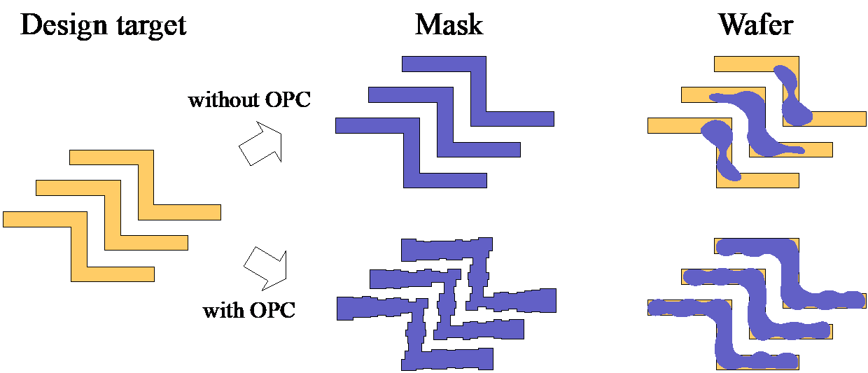
The introduction of GANs has paved the way for a new class of models that stemmed from the original GAN concept. In fact, different versions of GANs, tailored towards specific domain and applications, were proposed especially for image related tasks. Among these are the CGANs which, in contrast with original GANs, learn a mapping from an observed image \(x\) and random noise vector \(z\), to \(y\), \(G : \left\{ x, z\right\} \to y\). Technically, CGANs have changed the objective from a pure generative one to a domain-transfer task capable of establishing a mapping between images in different domains. Its applications span different domains ranging from image coloring to aerial to map, edge to photo translations, and medical applications among others ^[29]. Looking at it abstractly, such models can be viewed in many fields as data-trained simulators or optimizers that can perform complex operations such as lithography simulation as shown in [15]. In fact, the CGAN model is the most adopted generative model for EDA applications ^{[15, 16, 18, 19, 21, 22]}.

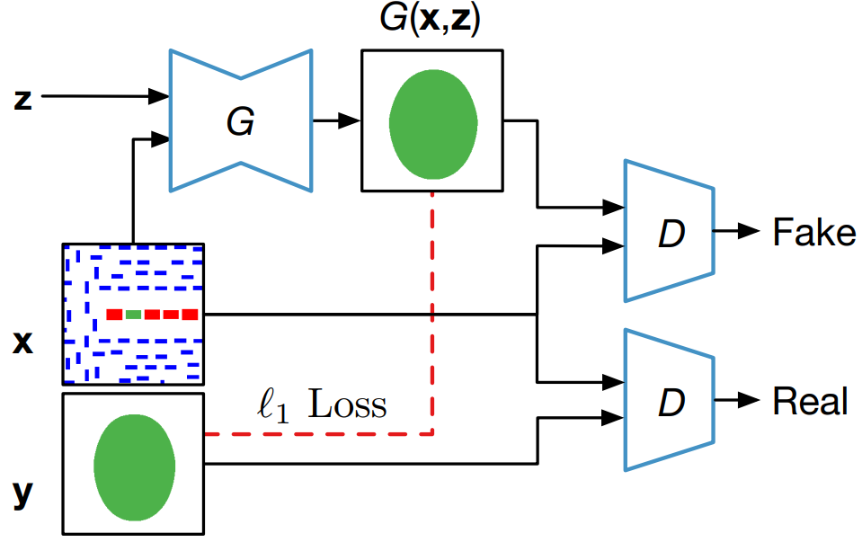
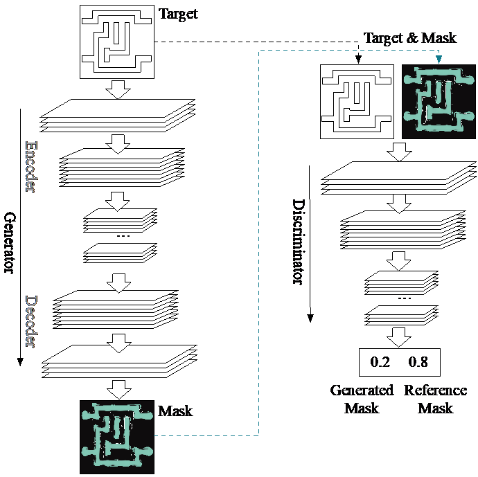
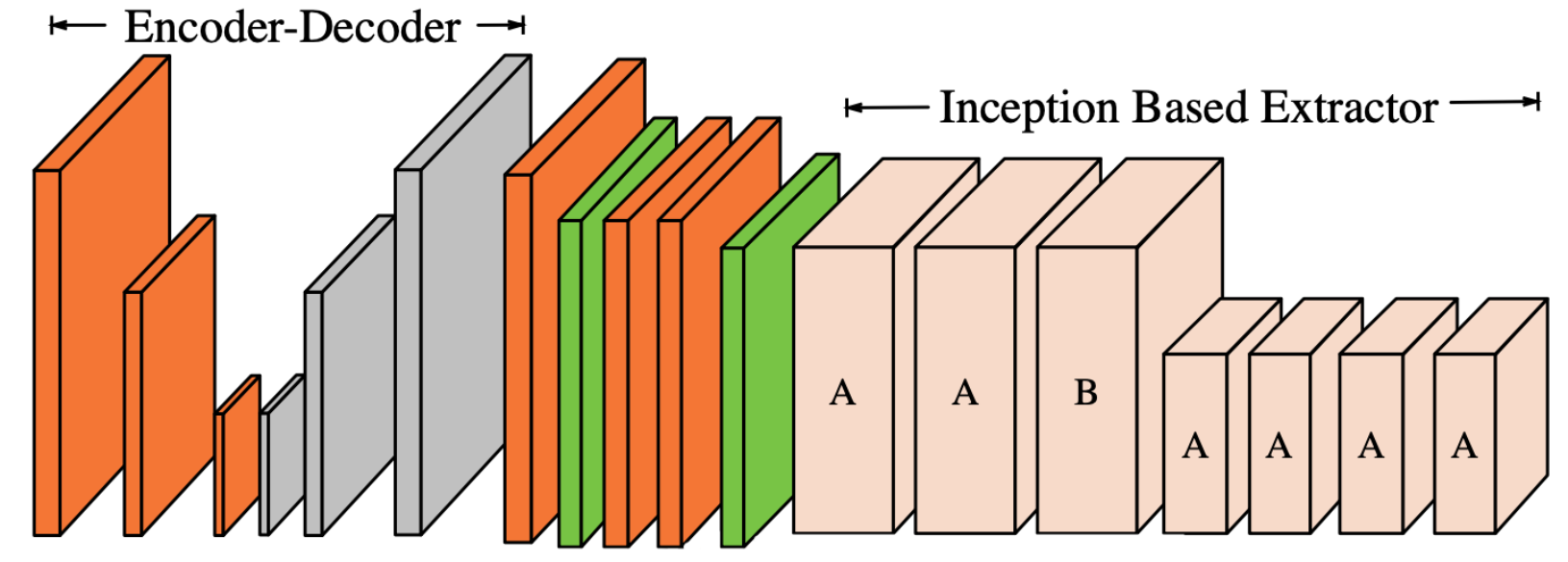
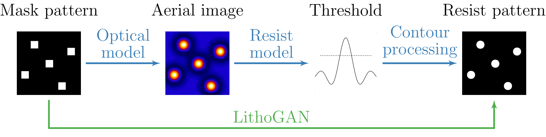
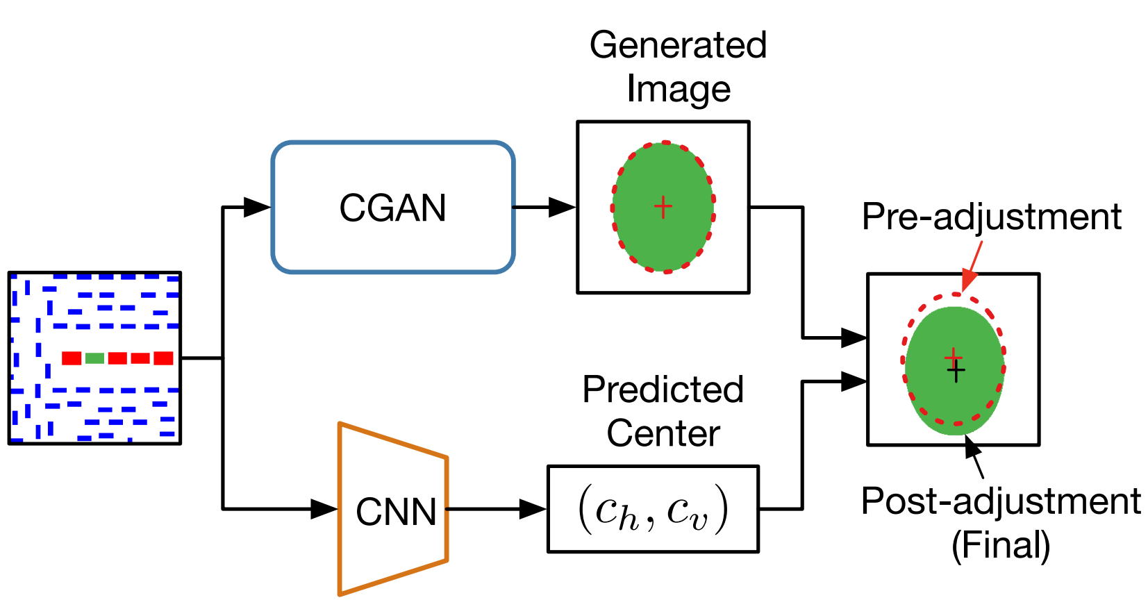
Figure 2. CGAN for lithography modeling^[15].

The architecture of the CGAN used for end-to-end lithography simulation is shown in Fig. 2 where \(G\) translate an image from the layout domain to the resist shape domain, and \(D\) examines image pairs to detect fake ones (further details about this application are presented in Section 3.3). Mathematically, one form of a loss function used for training the CGAN can be given as ^{[10, 29]}:

\[{\mathcal{L}}_{CGAN}\left(G,D\right)={\mathbb{E}}_{x,y}\left[logD\left(x,y\right)\right]+{\mathbb{E}}_{x,z}\left(log\left[1-D\left(x,G\left(x,z\right)\right)\right]\right)+\lambda {\mathbb{E}}_{x,z,y}l\left(y,G\left(x,z\right)\right)\qquad \qquad \qquad \text{(5)}\]

where \(x\) is a sample in the input domain and \(y\) is its corresponding sample in the output domain. Comparing equations (4) and (5), one can notice the addition of the loss term which penalizes the difference between the generated sample G(\(x\), \(z\)) and its corresponding golden reference \(y\). Different loss functions are adopted in different CGAN models including l₁ -norm and l₂ -norm

3. Generative Learning in Design for Manufacturability

Lithography is one of the key stages in VLSI manufacturing. In advanced technology nodes, two lithography related steps, mask synthesis and verification, become extremely time consuming due to the complicated lithography systems and demands to high resolution. In this section, we will introduce how generative learning helps accelerate lithography steps and facilitates design closure.

3.1 GAN-OPC

With the continuous scaling of VLSI technology, the mask optimization process becomes a great challenge for designers. Resolution enhancement techniques (RETs) are critical for obtaining high manufacturing quality and yield. Among these techniques, optical proximity correctness (OPC) plays a pivotal role in improving mask printability^{[30, 31]}. In particular, OPC aims at compensating lithography proximity effects through correcting mask pattern shapes as shown in Fig. 3.

Figure 3. Motivation of OPC^{[4, 32]}.

Conventional OPC methodologies are mostly model based where pattern edges are fractured into segments that are then shifted/corrected according to mathematical models^[33]. While such an approach can generate high quality results, it requires iterative and massive calls of expensive lithography simulation^[33]. To improve the efficiency of OPC, regression based approaches have been proposed to achieve fast full-chip OPC with acceptable performance loss^[30–32].

In these approaches, design targets are fragmented, and features extracted from the fragmented layout are used for regression model training. However, and due to the complicated optical proximity effects, the regression models need to be complex; hence, they are prone to major over-fitting issues which limit their generalizability.

To overcome the over-fitting issue, Matsunawa et al^[34] proposed a hierarchical Bayes model (HBM) with concentric circular area sampling (CCAS) as the feature extraction technique. HBM trains a generalized linear mixed model to consider various edge types, including normal, convex, concave, and line-end edge, by regarding each edge type as a random effect with a random variance. As a result, HBM is capable of generating solutions with comparable quality to that from 10 iterations of conventional model-based approach, with a significant reduction in runtime. With such a performance, HBM was utilized to obtain a good starting point for model based OPC to reduce the number of required iterations and hence speedup the convergence.

Recently, Yang et al^[22]presented GAN-OPC, as a first generative learning-based approach for OPC leveraging a CGAN framework^[35]. The key idea is to cast the mask generation task as a domain transfer problem where the objective is to map a ‘Target’ pattern to its corresponding ‘Mask’ pattern as shown in Fig. 4. The architecture of GAN-OPC is shown in Fig. 4 which, as discussed in Section 2.2, comprises two network models: a generator and a discriminator. The generator has an auto-encoder structure^[36], which takes a design target as an input in an image format and outputs a mask clip. On the other hand, the discriminator is a classifier that differentiates generated masks and reference masks. In practice, the core OPC operation lies in the generator which learns a mapping function that can capture the mask optimization process whereas the discriminator helps guide the learning process during training.

Figure 4. Neural network architecture of GAN-OPC^[22].

In the training process, the loss function in Equation (5) is used with an l₂ -norm loss between the golden and generated mask images^[22]. Such a loss function can be optimized with various stochastic gradient descent algorithms^[37]. After training, GAN-OPC is used to provide the starting point for a conventional ILT engine^[38], as shown in Fig. 5. Compared with conventional ILT, GAN-OPC flow is reported to achieve 9% reduction in edge placement error (EPE) error, 1% reduction in process variation (PV) band, and over 2× reduction in the overall runtime. The runtime for the generator inference is only around 0.05% of the entire runtime. GAN-OPC not only speedups the convergence of ILT, but also improves the solution quality. Hence, generative learning was used in this application as an optimizer rather than a typical model used for regression or classification task, and it is evident that it can perform a good job in terms of both performance and speedup.

Figure 5. GAN-OPC flow ^[22].

3.2 GAN-SRAF

Similar to OPC, sub-resolution assist feature (SRAF) generation is a key RET to improve the target pattern quality and lithographic process window. These assist features are not actually printed; instead, the SRAF patterns would deliver light to the positions of target patterns at proper phase which can improve the robustness of target printing to lithographic variations^[39].

In literature, different SRAF generation approaches have been proposed and adopted. On one hand, there are rule-based approaches that can achieve acceptable accuracy within short execution time for simple designs and regular target patterns; yet fall short of handling complex shapes ^{[40, 41]}. On the other hand, model-based SRAF generation methods have been proposed relying on either simulated aerial images to seed the SRAF generation^{[42, 43]}, or inverse lithography technology (ILT) to compute the image contour and guide the SRAF generation^[44]. Despite better lithographic performance compared to the rule-based approach, the model-based SRAF generation is very time-consuming^[39].

Xu et al ^[39] introduced machine learning to tackle the problem of SRAF insertion more efficiently ^{[4, 39]}. The proposed method relies on SRAF features extraction with local sampling scheme to obtain the optimal SRAF map. This approach has achieved 10x speedup compared to model-based approaches with comparable quality^[39].

Figure 6. Multi-channel heatmaps encoding process where (a) shows an original layout representation and (b) shows the encoded representation^[21].

Recently, Alawieh et al^[21]proposed GAN-SRAF that leverages generative adversarial learning to further improve the efficiency of SRAF insertion problem by examining it from a new perspective. In fact, a layout can be simply viewed as an image; hence, machine learning techniques developed for image related tasks can come in handy. Specifically, CGANs have been adopted to perform a wide range of domain transfer tasks where image translation is the most infamous^{[10, 29]}. Hence, the SRAF generation task is cast into an image translation task where the two images domains are: (i) original layout and (ii) layout with SRAFs. Thus, generating an SRAF scheme for a particular layout can be seen as translating the layout image from the first domain (i.e., original layout) to the second domain (i.e., layout with SRAFs)^{[21, 29]}.

However, direct image representation of layout is not suitable for the SRAF generation using GANs due to two major limitations. First, GANs exhibit inherent limitation in detecting sharp edges and are not guaranteed to generate “clean” rectangular shapes for the SRAFs^[45]. In addition, extracting the SRAF information from the image to be mapped back to the layout file can be prohibitively expensive. Hence, a special encoding scheme, typically used in keypoint estimation^[46–49], is proposed in [21] to overcome the aforementioned limitations. The proposed scheme is based on multi-channel heatmaps which associates each object type with one channel in the image^{[48, 49]}. An example of such encoding is shown in Fig. 6 where an original layout is shown in Fig. 6 (a) and the multi-channel heatmap representation is shown in Fig. 6 (b). In this example, the number of channels is set to 3 to visualize the encoded representation through a red-green-blue (RGB) image: (i) target patterns (in red), (ii) horizontal SRAFs (in green) and (iii) vertical SRAFs (in blue).

The encoding has two main advantages: (i) no sharp edges in the image representation, and (ii) images generated by the GAN models can be easily mapped back to layout files using a fast custom CUDA accelerator for the decoding scheme ^[21]. The overall GAN-SRAF framework is based upon a CGAN model for domain transfer as shown in Fig. 7.

Figure 7. GAN-SRAF overall flow^[21].

Results presented in [21] show that GAN-SRAF can achieve 14× reduction in runtime compared to the work in [39] and 144× when compared to model-based approaches while achieving comparable results. Here again, generative learning was utilized to efficiently perform an end-to-end RET task to optimize the lithography process.

3.3 LithoGAN

During the lithography process, a designed mask pattern is transferred into a resist pattern on the top surface of a semiconductor wafer^{[50, 51]}. The semiconductor industry has relied on lithography simulation for process development and performance verification. Rigorous lithography simulation precisely simulates the physical effects of materials but is computationally expensive. Therefore, compact models stand as a speedup alternative to rigorous computation with a small sacrifice in accuracy, which enables its wide application for lithography verification.

Fig. 8 shows a typical flow of lithography simulation. First, an aerial image is calculated from a mask pattern using a compact optical model. Then a resist model is used to determine the locally varying slicing thresholds^[52]. The thresholds are processed through extrapolation together with the corresponding aerial image to evaluate the critical dimension (CD) of the printed patterns.

Figure 8. Conventional lithography simulation flow consisting of multiple stages and the proposed LithoGAN flow ^[15].

Machine learning-based techniques have been proposed as a substitute for compact models for better simulation quality^{[4, 53–55]}. [53] proposed an artificial neural network (ANN) for resist height prediction. [54] proposed a convolutional neural network (CNN) model that predicts the slicing thresholds in aerial images accurately. Recently, [55] proposed a transfer learning model to cope with the deficiency in the manufacturing data at advanced technology nodes.

These machine learning-based resist modeling techniques still suffer from an exorbitant computational cost while providing partial modeling schemes that rely heavily on pre and post-processing procedures. For this purpose, Ye et al.^[15] proposed an end-to-end lithography modeling framework, LithoGAN, to directly map mask patterns to resist patterns by utilizing CGAN. The input domain is the mask designs converted to RGB images, where the target contact of interest is encoded into the green channel, neighboring contacts are encoded into the red channel, and SRAFs are encoded into the blue channel as shown in Fig. 9. The output of CGAN is the zoomed-in resist patterns corresponding to the center contact.

Figure 9. LithoGAN framework^[15].

For traditional computer vision tasks, locations of the objects in the generated image are not a major concern. For example, when trained on car images, the output of the GAN is judged upon based on the quality of an image as seen by a human while neglecting the exact location of the car in the image. However, for the lithography modeling task, the location of the generated resist pattern is as important as the shape of the pattern.

Therefore, as illustrated in Fig. 9, there are two data paths in LithoGAN, where the shape and the location of the resist pattern are predicted separately. In the first path, a trained CGAN model is utilized to predict the shape of the resist pattern. During training, the golden pattern is re-centered at the center of the image, and the coordinates of the original center are saved for CNN training. In other words, the model is trained to predict resist patterns that are always centered at the center of the images. On the other hand, the second path is composed of a CNN trained to predict the center of the resist pattern based on the mask image. Here the center refers to the center of the bounding box enclosing the resist pattern. They are combined in the last step before output: the image generated by CGAN is adjusted by recentering the resist shape based on center the coordinates predicted from the CNN.

Experimental results reported in [15] demonstrates that LithoGAN can achieve ∼1800× runtime reduction when compared to rigorous simulation, while obtaining resist pattern results that fall within the accepted lithography range.

3.4 Layout Generation

Most applications in previous sections are domain translation tasks, where the model is given an input from one domain and generates the output in another domain. In this section, we introduce a different task: pattern generation. In advanced manufacturing, various patterns are required to validate the manufacturing process. However, generating meaningful patterns is not an easy task, due to complicated design rules and high demands of pattern diversity. Figure 10 shows an example of design rules for EUV lithography.

Figure 10. Layout rules under EUV lithography^[23].

Figure 11. Squish representation for layout patterns ^[23].

To tackle this challenging task, Yang et al^[23]proposed a DeePattern framework to generate high-quality random patterns following the design rules with high pattern complexity and diversity. They divide the task into two steps: topology generation and legal pattern generation. These two steps are realized with the squish representation for layout patterns, as shown in Fig. 11, where T specifies the topology and δ_x, δ_y indicate the concrete width/length and spacing. As the topology T is essentially a matrix, generative models can be adopted for the topology generation, such as the transforming convolutional auto-encoder proposed in DeePattern. By perturbation to the latent space of the autoencoder, random topology can be obtained. With the generated topology matrix T, a legal δ_x, δ_y pair can be obtained by solving a linear system with constraints to clip sizes and design rules as follows:

\[\begin{array}{cc}{y}_{i+1}-{y}_{i}=\frac{p}{2}& \forall i\end{array} \qquad\qquad\text{(6a)}\\ \begin{array}{cc}{x}_{i}-{x}_{j}={t}_{min}& \forall \left(i,j\right)\in {S}_{T2T}\end{array} \qquad\text{(6b)}\\ \begin{array}{cc}{x}_{i}-{x}_{j}={l}_{min}& \forall \left(i,j\right)\in {S}_{L}\end{array} \qquad\text{(6c)}\\ \begin{array}{cc}{x}_{i+1}-{x}_{i}>0& \forall i\end{array} \qquad\qquad\text{(6d)}\\ \begin{array}{cc}{x}_{max}-{x}_{0}={d}_{x}& \end{array} \qquad\qquad\text{(6e)}\\\begin{array}{cc}{y}_{max}-{y}_{0}={d}_{y}& \end{array}\qquad\qquad\text{(6f)}\]

where p denotes the pitch in Fig. 10, t_min denotes the minimum tip-to-tip spacing, l_min denotes the minimum length, d_x and d_y denote the clip sizes. The set S_T2T represents the scan lines for minimum tip-to-tips in the topology and the set S_L represents that for minimum line segments.

It needs to be noted that the autoencoder may generate illegal topology such as 2D shapes, bow-tie-like shapes, and segments covering multiple tracks, these results are omitted with a legality check. To increase the diversity of the patterns, DeePattern measures the sensitivity of each dimension in the latent codes and adds Gaussian noise to proper dimensions. Fig. 12 shows an example generated from the state-of-the-art industry tool, DCGAN, and DeePattern. It can be seen that DeePattern generates much closer topologies to the industry tool. Fig. 13 also demonstrates that DeePattern achieves better diversity than the industry tool.

Figure 12. Sample pattern topology from (a) Industry tool, (b) DCGAN, and (c) DeePattern^[23].

Figure 13. Distributions of layout generation: (a) industrial tool and (b) DeePattern^[23].

3.5 Lithography Hotspot Detection

Traditionally, lithography hotspots were accurately detected through full-chip lithography simulations which compute the aerial images and contours of printed patterns^{[56, 57]}; though, at a tremendous computational cost. However, this task has recently received significant attention after machine learning technique were leveraged with remarkable success^{[25, 58–61]}. In particular, different deep learning models have been proposed to address this problem with the target of detecting whether a given layout clip is a lithography hotspot or not, hence, casting the problem as a binary classification task. However, addressing this task is not trivial. Despite the fact that the lithography defects are critical, their relative number is significantly small across the whole chip due to the highly imbalance nature of the data. Thus, different approaches have been proposed to achieve high accuracy hotspot detection through addressing the data imbalance challenge^{[59, 60]}.

Recently, Chen et al^[25] have examined the hotspot detection problem from a new angle. Different from the traditional approaches, the hotspot detection problem is cast as an object detection task rather than a binary classification one. In other words, instead of dividing the layout into different clips and predicting a binary label for each using machine learning models, an entire layout region is considered where the task is to detect all hotspots in the region^[25].

The approach proposed in [25] comprises a multi-stage deep learning model including: (i) feature extraction, (ii) clip proposal network, and (iii) refinement. Relevant to our discussion is the implementation of the feature extractor which is based upon an autoencoder framework. As discussed in Section II, autoencoders were developed as a tool for feature extraction and data compression. In [25], and unlike previous works on hotspot detection where features were pre-set such as using Discrete Cosine Transform (DCT) in [60], feature extraction is data driven. With the AE scheme, the model optimizes for the feature extraction as a part of the overall hotspot detection framework. The feature extraction scheme used in [25] is shown in Fig. 14 which contains an autoencoder scheme along with an inception model.

This feature extraction scheme is followed by a two-stage classification and regression framework which can achieve significant reduction in prediction runtime and better performance in terms of both hotspot detection accuracy and false alarms^[25]. Thus, generative learning is utilized in this work to provide a self-adaptive feature transformation scheme that is very compatible with convolution neural networks and time saving^[25].

It is worth mentioning that the adversary nature of GAN has been recently used to study the resilience of machine learning models against adversarial perturbation. In [24], Liu et at studied the potential of adversary attacks on machine learning based EDA approaches while considering hotspot detection as a case study. The study showed that CNN-based hotspot detectors can be fooled by specially crafted SRAF insertions that can mislead the network to predict a hotspot layout as non-hotspot. This first study unearthed a threat that should be considered when using machine leaning tools in EDA, thus, urging caution and advocating for further study of the wider security implications of deep learning in this field^[24].

Figure 14. Feature extractor for hotspot detection using autoencoder^[25].

4. General Takeaways

The aforementioned applications of generative learning in the field of DFM represent a part of a new paradigm in the field based on machine learning. In general, the driving motivation for this new path is enhancing performance and speeding up design closure. However, generative learning has left its unique characteristics.

• Design Representation: When using generative learning, design representations at different stages are cast into visual context, i.e., designs or layouts are treated as images. While such visual representations are not trivial in some cases, as in the case of the SRAF encoding scheme in Section 3.2, it has been shown that, if an adequate representation can be obtained, a wide range of models and tools are available to handle different applications. In practice, new machine learning models for computer vision are developed continuously and generative learning is one of the latest. Thus, providing competent visual representation for designs at different levels is the first step towards using the resourceful machine learning toolbox for computer vision as shown in the examples presented in Section 3.

• Models as Optimizers: While conventional machine learning models are viewed in the scope of regression and classification tools, generative learning has taken that one step further to act as a stand-alone simulator as in LithoGAN (Section 3.3) and as an optimizer in both GAN-OPC and GAN-SRAF (Sections 3.1 and 3.2). In practice, these generative models are now generating solutions that can parallel those of conventional tools and are doing that much faster. For example, with 1800× speedup in lithography simulation, LithoGAN is redefining the role of machine learning in lithography. Therefore, it is expected that such models will be introduced into different early exploration stages in DFM resulting in orders of magnitude speedup compared to traditional approaches; hence, revolutionizing the way the field is perceived

• Adversary in ML for DFM: While most generative adversarial models have used adversary towards good ends, it is important to keep in mind that it is still called adversarial for a reason, and it can be used towards different ends. In Section 3.5, the adversary threat for ML models was briefly introduced, and this topic is expected to attract more attention as adoption of ML techniques expands. Here, generative models can be used to build more resilient ML models that are capable of withstanding adversarial attacks.

5. Conclusion

This paper reviews the recent generative learning applications in various design for manufacturability tasks, such as lithography modeling, hotspot detection, and mask optimization. While conventional approaches to address these tasks are data intensive and computationally expensive, generative learning is emerging as an alternative framework that can substitute them while improving performance and/or efficiency, eventually contributing to fast design closure and good manufacturability. In fact, generative learning has stepped out of the conventional frame for ML models to act as a data-driven optimizer or simulator that can significantly speedup design closure. This paves the way for a new paradigm of design automation with limited dependence on expensive traditional simulation and optimization tools.

With the proven success in many DFM applications, wider adoption of these models still faces some challenges:

• requirement of high resolution in many accuracy demanding applications;

• adequate visual representation for target designs and applications;

• requirement of large initial training datasets;

• requirement of framework for data re-use when technology changes.

These challenges are already under spotlight for research in machine learning where new solutions are being developed to overcome them in ML applications in different fields. With more success at this front in the near future, wider adoption of generative learning in EDA, and DFM in particular, is expected.

Acknowledgments

This work is supported in part by NSF under Award No. 1718570 and Kioxia.

[1] M. Fatima and M. Pasha, “Survey of machine learning algorithms for disease diagnostic,” Journal of Intelligent Learning Systems and Applications, vol. 9, no. 01, p. 1, 2017.